本文仅供学习使用
本文参考:
B站:CLEAR_LAB
笔者带更新-运动学
课程主讲教师:
Prof. Wei Zhang
课程链接 :
https://www.wzhanglab.site/teaching/mee-5114-advanced-control-for-robotics/
南科大高等机器人控制课 Ch11 Bascis of Optimization
- 1. Motivation
- 2. Some Linear Algebra
- 2.1 Real Symmetric Matrices
- 2.2 Positive Semidefinite Matrices
- 3. Set and Functions
- 3.1 Affine Sets and Functions
- 3.2 Qyadratic Sets and Functions
- 3.3 Convex Set
- 3.4 Cone
- 3.5 Positve Semidefinite Cone
- 3.6 Operations that Preserve Convexity
- 3.7 Convex Function
- 3.8 How to Check a Function of Convex?
- 3.9 Example of Convex Functions
- 4. Short Introduction to Optimization
- 4.1 Nonlinear Optimiazation Problems
- 4.2 Lagrangian
- 4.2.1 Lagrangian Dual Problems
- 4.2.2 Duality Theorems
- 4.3 General Optimality Conditions
- 4.4 KKT Conditions
- 5. Linear Program
- 6. Quadratic Program
1. Motivation
Optimization is argulably the most important tool for modern engineering
Robotics:
- Differential Inverse Kinematics
- Dynamics :
ABA(most efficient dynamics algorithm) andLQR - Motion planning
- Whole-body control: formulated as a quadratic program
- SLAM
- Preception
Machine Learning
- Linear regression
- Support vector machine
- Deep learning —— minimize ‘loss’ function
Other domains
- Check system stability : SDP
- Compressive sensing
- Fourier transform : keast square problem
Roughly speaking, most engineering problems (finding a better design, ensure certain properties of the solution, develop an algorithm), can be formulated as optimization / optimal control problems.

Our goal :
- Basic knowledge/key concepts of opt. theory
- Formulate / Reformulate opt. problem
- Educated users of tools/packages
2. Some Linear Algebra
2.1 Real Symmetric Matrices
S n ∈ R n × n \mathcal{S} ^n\in \mathbb{R} ^{n\times n} Sn∈Rn×n : set of real symmetric matrices in R n \mathbb{R} ^n Rn , A ∈ S n ⇔ A T = A A\in \mathcal{S} ^n\Leftrightarrow A^{\mathrm{T}}=A A∈Sn⇔AT=A
All eigenvalues are real (diagonalizable) —— Important
There exists a full set of orthogonal eigenvectors A ∈ S n , A = T Λ T − 1 A\in \mathcal{S} ^n,A=T\varLambda T^{-1} A∈Sn,A=TΛT−1 nonsigular matrix
Spectral decomposition : If A ∈ S n A\in \mathcal{S} ^n A∈Sn , then A = Q Λ Q − 1 A=Q\varLambda Q^{-1} A=QΛQ−1 , where Λ \varLambda Λ diagonal and Q Q Q is unitary —— Q T Q = E Q^{\mathrm{T}}Q=E QTQ=E Q = [ q 1 , . . . , q n ] Q=\left[ q_1,...,q_{\mathrm{n}} \right] Q=[q1,...,qn] q i q_{\mathrm{i}} qi is i i ith-column of Q Q Q —— ⇒ q i T q j = { 0 i = j 1 o t h e r w i s e \Rightarrow {q_{\mathrm{i}}}^{\mathrm{T}}q_{\mathrm{j}}=\begin{cases} 0 i=j\\ 1 otherwise\\ \end{cases} ⇒qiTqj={0i=j1otherwise , { q i } \left\{ q_{\mathrm{i}} \right\} {qi} orthonormal
2.2 Positive Semidefinite Matrices
A ∈ S n A\in \mathcal{S} ^n A∈Sn is called positive semidefinite(PSD), denoted by A ⪰ 0 A\succeq 0 A⪰0 , if x T A x ⩾ 0 , ∀ x ∈ R n x^{\mathrm{T}}Ax\geqslant 0,\forall x\in \mathbb{R} ^n xTAx⩾0,∀x∈Rn
A ∈ S n A\in \mathcal{S} ^n A∈Sn is called positive definite(PD) , denoted by A ≻ 0 A\succ 0 A≻0 , x T A x > 0 x^{\mathrm{T}}Ax>0 xTAx>0 for all nonzero x ∈ R n x\in \mathbb{R} ^n x∈Rn
S + n \mathcal{S} _{+}^{n} S+n : set of all PSD (symmetric) matrices
S + + n \mathcal{S} _{++}^{n} S++n : set of all PD (symmetric) matrices
PSD or PD matrices can also be defined for non-symmetric matrices : e.g. [ 1 1 − 1 1 ] ⇒ x T [ 1 1 − 1 1 ] x = x 1 2 + x 2 2 \left[ \begin{matrix} 1& 1\\ -1& 1\\ \end{matrix} \right] \Rightarrow x^{\mathrm{T}}\left[ \begin{matrix} 1& 1\\ -1& 1\\ \end{matrix} \right] x={x_1}^2+{x_2}^2 [1−111]⇒xT[1−111]x=x12+x22
We assume PSD and PD are symmetric (unless otherwise noted)
Notation : A ⪰ B A\succeq B A⪰B (resp. A ≻ B A\succ B A≻B) means A − B ∈ S + n A-B\in \mathcal{S} _{+}^{n} A−B∈S+n (resp. A − B ∈ S + + n A-B\in \mathcal{S} _{++}^{n} A−B∈S++n) —— A − B A-B A−B PSD - defined a partial order on S n \mathcal{S} ^n Sn —— It is possible to have A ⊁ B , A ⋡ B A\nsucc B,A\nsucceq B A⊁B,A⋡B
Other equivalent definitions for symmetric PSD matrices :
- All 2 n − 1 2^n-1 2n−1 principal minors of A A A are nonnegative
- All eigs of A A A are nonnegative
- There exists a factorization A = B T B A=B^{\mathrm{T}}B A=BTB
Other equivalent definitions for symmetric PD matrices :
- All n n n principal minors of A A A are positive
- All eigs of A A A are strictly positive
- There exists a factorization A = B T B A=B^{\mathrm{T}}B A=BTB with B B B square and nonsingular
If A > 0 A>0 A>0 , A = Q Λ Q T = Q Λ 1 2 Λ 1 2 Q T = B T B , B = Λ 1 2 Q T A=Q\varLambda Q^{\mathrm{T}}=Q\varLambda ^{\frac{1}{2}}\varLambda ^{\frac{1}{2}}Q^{\mathrm{T}}=B^{\mathrm{T}}B, B=\varLambda ^{\frac{1}{2}}Q^{\mathrm{T}} A=QΛQT=QΛ21Λ21QT=BTB,B=Λ21QT
Useful facts :
-
If T T T nonsigular(doesn’t need to unitary) , A ≻ 0 ⇔ T T A T ≻ 0 A\succ 0\Leftrightarrow T^{\mathrm{T}}AT\succ 0 A≻0⇔TTAT≻0 and A ⪰ 0 ⇔ T T A T ⪰ 0 A\succeq 0\Leftrightarrow T^{\mathrm{T}}AT\succeq 0 A⪰0⇔TTAT⪰0
Recall : T A T − 1 TAT^{-1} TAT−1 : similarity transformation S + n \mathcal{S} _{+}^{n} S+n ; T T A T T^{\mathrm{T}}AT TTAT: congruent transformation S + + n \mathcal{S} _{++}^{n} S++n —— are invariant under congruent transformation -
Inner product on R m × n \mathbb{R} ^{m\times n} Rm×n : < A , B > = t r ( A T B ) = A ⋅ B <A,B>=tr\left( A^{\mathrm{T}}B \right) =A\cdot B <A,B>=tr(ATB)=A⋅B
∀ A ∈ R m × n , B ∈ R m × n t r ( A T B ) = ∑ i = 1 m ∑ j = 1 n A i j B i j \forall A\in \mathbb{R} ^{m\times n},B\in \mathbb{R} ^{m\times n}\,\,tr\left( A^{\mathrm{T}}B \right) =\sum_{i=1}^m{\sum_{j=1}^n{A_{\mathrm{ij}}B_{\mathrm{ij}}}} ∀A∈Rm×n,B∈Rm×ntr(ATB)=∑i=1m∑j=1nAijBij , Angle between A , B A,B A,B cos θ = < A , B > < A , A > < B , B > , { A ⊥ B ⇒ t r ( A T B ) = 0 t r ( A T B ) > 0 ⇒ a c u t e \cos \theta =\frac{<A,B>}{\sqrt{<A,A><B,B>}},\begin{cases} A\bot B\Rightarrow tr\left( A^{\mathrm{T}}B \right) =0\\ tr\left( A^{\mathrm{T}}B \right) >0\Rightarrow acute\\ \end{cases} cosθ=<A,A><B,B><A,B>,{A⊥B⇒tr(ATB)=0tr(ATB)>0⇒acute -
For A , B ∈ S + n , t r ( A B ) > 0 A,B\in \mathcal{S} _{+}^{n},tr\left( AB \right) >0 A,B∈S+n,tr(AB)>0 —— A , B A,B A,B square symmetric PSD : < A , B > = t r ( A T B ) = t r ( A B ) ⇒ t r ( A B ) ⩾ 0 <A,B>=tr\left( A^{\mathrm{T}}B \right) =tr\left( AB \right) \Rightarrow tr\left( AB \right) \geqslant 0 <A,B>=tr(ATB)=tr(AB)⇒tr(AB)⩾0
-
For ant symmetric A ∈ S n A\in \mathcal{S} ^n A∈Sn , λ min ( A ) ⩾ μ ⇔ A ⪰ μ E \lambda _{\min}\left( A \right) \geqslant \mu \Leftrightarrow A\succeq \mu E λmin(A)⩾μ⇔A⪰μE and λ max ( A ) ⩽ β ⇔ A ⪯ β E \lambda _{\max}\left( A \right) \leqslant \beta \Leftrightarrow A\preceq \beta E λmax(A)⩽β⇔A⪯βE (easy proof)
3. Set and Functions
3.1 Affine Sets and Functions
Linear mapping : f ( x + y ) = f ( x ) + f ( y ) , f ( α x ) = α f ( x ) f\left( x+y \right) =f\left( x \right) +f\left( y \right) ,f\left( \alpha x \right) =\alpha f\left( x \right) f(x+y)=f(x)+f(y),f(αx)=αf(x) , for any x , y x,y x,y in some vector space , and α ∈ R \alpha \in \mathbb{R} α∈R
Examples:
- f ( x ) = A x , x ∈ R 3 , A ∈ S O ( 3 ) f\left( x \right) =Ax,x\in \mathbb{R} ^3,A\in SO\left( 3 \right) f(x)=Ax,x∈R3,A∈SO(3)
- f ( x ) = ∫ x ( τ ) d τ f\left( x \right) =\int{x\left( \tau \right) d\tau} f(x)=∫x(τ)dτ , for all integrable function x ( ⋅ ) x\left( \cdot \right) x(⋅)
- E ( x ) E\left( x \right) E(x) expection of random variable/vector x x x —— E ( x ) = ∫ x f ( x ) d x E\left( x \right) =\int{xf\left( x \right) dx} E(x)=∫xf(x)dx
- f ( x ) = t r ( x ) , x ∈ R n × n f\left( x \right) =tr\left( x \right) ,x\in \mathbb{R} ^{n\times n} f(x)=tr(x),x∈Rn×n
Affine mapping : f ( x ) f\left( x \right) f(x) is an affine mapping of x x x if g ( x ) = f ( x ) − f ( x 0 ) g\left( x \right) =f\left( x \right) -f\left( x_0 \right) g(x)=f(x)−f(x0) is a linear mapping for some fixed x 0 x_0 x0
Finite-deimension representation fo affine function : f ( x ) = A x + b f\left( x \right) =Ax+b f(x)=Ax+b —— g ( x ) = f ( x ) − f ( 0 ) = A x + b − b = A x g\left( x \right) =f\left( x \right) -f\left( 0 \right) =Ax+b-b=Ax g(x)=f(x)−f(0)=Ax+b−b=Ax
Homogeneous representation in R n \mathbb{R} ^n Rn : f ( x ) = A x + b ⇔ f ^ ( x ) = A ^ x ^ , A ^ = [ A b 0 1 ] , x ^ = [ x 1 ] f\left( x \right) =Ax+b\Leftrightarrow \hat{f}\left( x \right) =\hat{A}\hat{x},\hat{A}=\left[ \begin{matrix} A& b\\ 0& 1\\ \end{matrix} \right] ,\hat{x}=\left[ \begin{array}{c} x\\ 1\\ \end{array} \right] f(x)=Ax+b⇔f^(x)=A^x^,A^=[A0b1],x^=[x1]
Linear and affine are often used interchangeably
Linear/affine sets: { x : f ( x ) ⩽ 0 } \left\{ x:f\left( x \right) \leqslant 0 \right\} {x:f(x)⩽0} ofr affine mapping f f f
- Line/hyperplane : a T x = b a^{\mathrm{T}}x=b aTx=b
a T x = b ⇒ a T ( x − x 0 ) = 0 ⇒ a T x − a T x 0 = 0 , a T x 0 = b a^{\mathrm{T}}x=b\Rightarrow a^{\mathrm{T}}\left( x-x_0 \right) =0\Rightarrow a^{\mathrm{T}}x-a^{\mathrm{T}}x_0=0,a^{\mathrm{T}}x_0=b aTx=b⇒aT(x−x0)=0⇒aTx−aTx0=0,aTx0=b - Half space : a T x ⩽ b a^{\mathrm{T}}x\leqslant b aTx⩽b —— a T x − a T x 0 ⩽ 0 a^{\mathrm{T}}x-a^{\mathrm{T}}x_0\leqslant 0 aTx−aTx0⩽0
- Polyhedron : H x ⩽ h Hx\leqslant h Hx⩽h —— H ∈ R m × n , x ∈ R n , h ∈ R m H\in \mathbb{R} ^{m\times n},x\in \mathbb{R} ^n,h\in \mathbb{R} ^m H∈Rm×n,x∈Rn,h∈Rm
[ H 1 T ⋮ H m T ] x ⩽ [ h 1 ⋮ h m ] \left[ \begin{array}{c} {H_1}^{\mathrm{T}}\\ \vdots\\ {H_{\mathrm{m}}}^{\mathrm{T}}\\ \end{array} \right] x\leqslant \left[ \begin{array}{c} h_1\\ \vdots\\ h_{\mathrm{m}}\\ \end{array} \right] H1T⋮HmT x⩽ h1⋮hm —— Imposes m m m inequality H i T x ⩽ h i {H_{\mathrm{i}}}^{\mathrm{T}}x\leqslant h_{\mathrm{i}} HiTx⩽hi —— half space - For matrix variable X ∈ R n × n X\in \mathbb{R} ^{n\times n} X∈Rn×n, t r ( A X ) ⩽ 0 tr\left( AX \right) \leqslant 0 tr(AX)⩽0 for given constant matrix A ∈ R n × n A\in \mathbb{R} ^{n\times n} A∈Rn×n is halfspace in R n × n \mathbb{R} ^{n\times n} Rn×n

3.2 Qyadratic Sets and Functions
Quadratic functions in R n \mathbb{R} ^n Rn : f ( x ) = x T A x + b T x + c , x = [ x 1 ⋮ x n ] , f : R n → R f\left( x \right) =x^{\mathrm{T}}Ax+b^{\mathrm{T}}x+c,x=\left[ \begin{array}{c} x_1\\ \vdots\\ x_{\mathrm{n}}\\ \end{array} \right] ,f:\mathbb{R} ^n\rightarrow \mathbb{R} f(x)=xTAx+bTx+c,x= x1⋮xn ,f:Rn→R
Quadratic functions (honogeneous form) : x ^ = [ x 1 ] , f ^ ( x ) = [ x 1 ] T [ A b 2 b 2 c ] [ x 1 ] \hat{x}=\left[ \begin{array}{c} x\\ 1\\ \end{array} \right] ,\hat{f}\left( x \right) =\left[ \begin{array}{c} x\\ 1\\ \end{array} \right] ^{\mathrm{T}}\left[ \begin{matrix} A& \frac{b}{2}\\ \frac{b}{2}& c\\ \end{matrix} \right] \left[ \begin{array}{c} x\\ 1\\ \end{array} \right] x^=[x1],f^(x)=[x1]T[A2b2bc][x1] —— f ^ ( x ) = x ^ T A ^ x ^ \hat{f}\left( x \right) =\hat{x}^{\mathrm{T}}\hat{A}\hat{x} f^(x)=x^TA^x^ ( A ∈ S + n ⇔ f ( x ) ⩾ 0 , ∀ x ∈ R n A\in \mathcal{S} _{+}^{n}\Leftrightarrow f\left( x \right) \geqslant 0,\forall x\in \mathbb{R} ^n A∈S+n⇔f(x)⩾0,∀x∈Rn) —— f f f - PSD f ( x ) > 0 f\left( x \right) >0 f(x)>0 for all x ≠ 0 x\ne 0 x=0 ; f ( x ) = 0 f\left( x \right) =0 f(x)=0 for all x = 0 x=0 x=0
Quadratic sets : { x ∈ R n : f ( x ) ⩽ 0 } \left\{ x\in \mathbb{R} ^n:f\left( x \right) \leqslant 0 \right\} {x∈Rn:f(x)⩽0} for some quadratic function f f f
eg1: Ball —— { x ∈ R n ∥ x − x c ∥ 2 ⩽ r c 2 } \left\{ x\in \mathbb{R} ^n\left\| x-x_{\mathrm{c}} \right\| ^2\leqslant {r_{\mathrm{c}}}^2 \right\} {x∈Rn∥x−xc∥2⩽rc2} ⇒ f ( x ) = ( x − x c ) T ( x − x c ) − r c 2 ⩽ 0 \Rightarrow f\left( x \right) =\left( x-x_{\mathrm{c}} \right) ^{\mathrm{T}}\left( x-x_{\mathrm{c}} \right) -{r_{\mathrm{c}}}^2\leqslant 0 ⇒f(x)=(x−xc)T(x−xc)−rc2⩽0
eg2 : Ellipsoid : { x ∈ R n ( x − x c ) T P − 1 ( x − x c ) ⩽ 1 , P ∈ S + + n } \left\{ x\in \mathbb{R} ^n\left( x-x_{\mathrm{c}} \right) ^{\mathrm{T}}P^{-1}\left( x-x_{\mathrm{c}} \right) \leqslant 1,P\in \mathcal{S} _{++}^{n} \right\} {x∈Rn(x−xc)TP−1(x−xc)⩽1,P∈S++n}
3.3 Convex Set
Convex Set : A set S S S is convex if any line segment stays in the set
x 1 , x 2 ∈ S ⇒ α x 1 + ( 1 − α ) x 2 ∈ S , ∀ α ∈ [ 0 , 1 ] ⇒ α 1 x 1 + α 2 x 2 , α 1 + α 2 = 1 , α 1 ⩾ 0 , α 2 ⩾ 0 x_1,x_2\in S\Rightarrow \alpha x_1+\left( 1-\alpha \right) x_2\in S,\forall \alpha \in \left[ 0,1 \right] \Rightarrow \alpha _1x_1+\alpha _2x_2,\alpha _1+\alpha _2=1,\alpha _1\geqslant 0,\alpha _2\geqslant 0 x1,x2∈S⇒αx1+(1−α)x2∈S,∀α∈[0,1]⇒α1x1+α2x2,α1+α2=1,α1⩾0,α2⩾0
- convex combination of x 1 , x 2 x_1,x_2 x1,x2

Convex combination of x 1 , . . . , x k x_1,...,x_{\mathrm{k}} x1,...,xk :
{ α 1 x 1 + α 2 x 2 + . . . + α k x k : α i ⩾ 0 , ∑ i α i = 1 } \left\{ \alpha _1x_1+\alpha _2x_2+...+\alpha _{\mathrm{k}}x_{\mathrm{k}}:\alpha _{\mathrm{i}}\geqslant 0,\sum_i{\alpha _{\mathrm{i}}}=1 \right\} {α1x1+α2x2+...+αkxk:αi⩾0,i∑αi=1}
Convex hull-凸包 : c o ‾ { S } \overline{co}\left\{ S \right\} co{S} set of all convex combinations of points in S S S
3.4 Cone
A set S S S is called a cone if λ > 0 , x ∈ S ⇒ λ x ∈ S \lambda >0,x\in S\Rightarrow \lambda x\in S λ>0,x∈S⇒λx∈S

Conic-圆锥的 combination of x 1 x_1 x1 and x 2 x_2 x2 : x = α 1 x 1 + α 2 x 2 , α 1 ⩾ 0 , α 2 ⩾ 0 x=\alpha _1x_1+\alpha _2x_2,\alpha _1\geqslant 0,\alpha _2\geqslant 0 x=α1x1+α2x2,α1⩾0,α2⩾0 —— c o n e ( x 1 , . . . , x k ) = { ∑ i α i x i : α i ⩾ 0 } cone\left( x_1,...,x_{\mathrm{k}} \right) =\left\{ \sum_i{\alpha _{\mathrm{i}}x_{\mathrm{i}}}:\alpha _{\mathrm{i}}\geqslant 0 \right\} cone(x1,...,xk)={∑iαixi:αi⩾0}
Convex cone:
- a cone that is convex
- equivalently,a set that contains all the conic combinations of points in the set
3.5 Positve Semidefinite Cone
The set of positive semidefinite matrices(i.e, S + n \mathcal{S} _{+}^{n} S+n is a convex cone and is referred to as the positive semidefinite(PSD) cone) —— S + n \mathcal{S} _{+}^{n} S+n : set of PSD A ∈ S + n ⇒ λ A ⩾ 0 ⇒ λ A ∈ S + n A\in \mathcal{S} _{+}^{n}\Rightarrow \lambda A\geqslant 0\Rightarrow \lambda A\in \mathcal{S} _{+}^{n} A∈S+n⇒λA⩾0⇒λA∈S+n S + n \mathcal{S} _{+}^{n} S+n is a cone
By definition : pick arbitrary A , B ∈ S + n A,B\in \mathcal{S} _{+}^{n} A,B∈S+n , α A + ( 1 − α ) B ∈ S + n , α ∈ [ 0 , 1 ] \alpha A+\left( 1-\alpha \right) B\in \mathcal{S} _{+}^{n},\alpha \in \left[ 0,1 \right] αA+(1−α)B∈S+n,α∈[0,1] ( ⇒ x T ( α A + ( 1 − α ) B ) x = α x T A x + ( 1 − α ) x T B x ⩾ 0 \Rightarrow x^{\mathrm{T}}\left( \alpha A+\left( 1-\alpha \right) B \right) x=\alpha x^{\mathrm{T}}Ax+\left( 1-\alpha \right) x^{\mathrm{T}}Bx\geqslant 0 ⇒xT(αA+(1−α)B)x=αxTAx+(1−α)xTBx⩾0)
Recall that if A , B ∈ S + n A,B\in \mathcal{S} _{+}^{n} A,B∈S+n , then t r ( A B ) ⩾ 0 tr\left( AB \right) \geqslant 0 tr(AB)⩾0 . This indicates that the cone S + n \mathcal{S} _{+}^{n} S+n is acute.
x 1 ∈ R n , x 2 ∈ R n x_1\in \mathbb{R} ^n,x_2\in \mathbb{R} ^n x1∈Rn,x2∈Rn
α 1 x 1 + α 2 x 2 \alpha _1x_1+\alpha _2x_2 α1x1+α2x2 linear combination
α 1 x 1 + α 2 x 2 \alpha _1x_1+\alpha _2x_2 α1x1+α2x2 α 1 ⩾ 0 , α 2 ⩾ 0 \alpha _1\geqslant 0,\alpha _2\geqslant 0 α1⩾0,α2⩾0 conic combination
α 1 x 1 + α 2 x 2 \alpha _1x_1+\alpha _2x_2 α1x1+α2x2 α 1 ⩾ 0 , α 2 ⩾ 0 \alpha _1\geqslant 0,\alpha _2\geqslant 0 α1⩾0,α2⩾0 α 1 + α 2 = 1 \alpha _1+\alpha _2=1 α1+α2=1 convex combination
3.6 Operations that Preserve Convexity
Intersection of possibly infinite number of convex sets is convex
eg: polyhedron —— H 1 T x ⩽ h 1 , H 2 T x ⩽ h 2 , [ H 1 T H 2 T ] x ⩽ [ h 1 h 2 ] {H_1}^{\mathrm{T}}x\leqslant h_1,{H_2}^{\mathrm{T}}x\leqslant h_2,\left[ \begin{array}{c} {H_1}^{\mathrm{T}}\\ {H_2}^{\mathrm{T}}\\ \end{array} \right] x\leqslant \left[ \begin{array}{c} h_1\\ h_2\\ \end{array} \right] H1Tx⩽h1,H2Tx⩽h2,[H1TH2T]x⩽[h1h2]
eg: PSD cone
Affine mapping f : R n → R m f:\mathbb{R} ^n\rightarrow \mathbb{R} ^m f:Rn→Rm (i.e. f ( x ) = A x + b f\left( x \right) =Ax+b f(x)=Ax+b)
- f ( X ) = { f ( x ) : x ∈ X } f\left( X \right) =\left\{ f\left( x \right) :x\in X \right\} f(X)={f(x):x∈X} is convex whenever X ⊆ R n X\subseteq \mathbb{R} ^n X⊆Rn is convex
e.g. : Ellipsoid : E 1 = { x ∈ R n : ( x − x c ) T P − 1 ( x − x c ) ⩽ 1 } E_1=\left\{ x\in \mathbb{R} ^n:\left( x-x_{\mathrm{c}} \right) ^{\mathrm{T}}P^{-1}\left( x-x_{\mathrm{c}} \right) \leqslant 1 \right\} E1={x∈Rn:(x−xc)TP−1(x−xc)⩽1} or E 2 = { x c + A u : ∥ u ∥ 2 ⩽ 1 } E_2=\left\{ x_{\mathrm{c}}+Au:\left\| u \right\| _2\leqslant 1 \right\} E2={xc+Au:∥u∥2⩽1} - f − 1 ( Y ) = { x ∈ R n : f ( x ) ∈ Y } f^{-1}\left( Y \right) =\left\{ x\in \mathbb{R} ^n:f\left( x \right) \in Y \right\} f−1(Y)={x∈Rn:f(x)∈Y} is convex whenever Y ⊆ R m Y\subseteq \mathbb{R} ^m Y⊆Rm is convex
e.g. { A x ⩽ b } = f − 1 ( R + n ) \left\{ Ax\leqslant b \right\} =f^{-1}\left( \mathbb{R} _{+}^{n} \right) {Ax⩽b}=f−1(R+n) , where R + n \mathbb{R} _{+}^{n} R+n in nonnegative orthant
3.7 Convex Function
Consider a finite dimensional vector space χ \chi χ . Let D ⊂ χ \mathcal{D} \subset \chi D⊂χ be convex
Definition 1 (Convex Function)
A function f : D → R f:\mathcal{D} \rightarrow \mathbb{R} f:D→R is called convex if
f ( α x 1 + ( 1 − α ) x 2 ) ⩽ α f ( x 1 ) + ( 1 − α ) f ( x 2 ) , ∀ x 1 , x 2 ∈ D , ∀ α ∈ [ 0 , 1 ] f\left( \alpha x_1+\left( 1-\alpha \right) x_2 \right) \leqslant \alpha f\left( x_1 \right) +\left( 1-\alpha \right) f\left( x_2 \right) ,\forall x_1,x_2\in \mathcal{D} ,\forall \alpha \in \left[ 0,1 \right] f(αx1+(1−α)x2)⩽αf(x1)+(1−α)f(x2),∀x1,x2∈D,∀α∈[0,1]
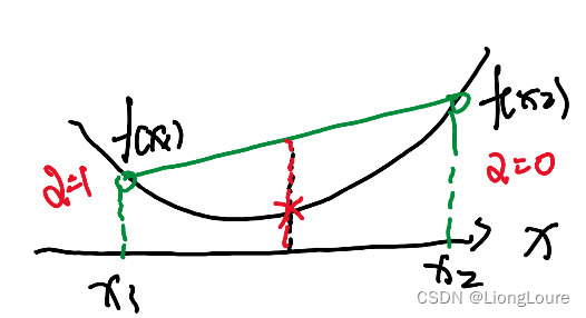
- f : D → R f:\mathcal{D} \rightarrow \mathbb{R} f:D→R is called strictly convex if
f ( α x 1 + ( 1 − α ) x 2 ) < α f ( x 1 ) + ( 1 − α ) f ( x 2 ) , ∀ x 1 ≠ x 2 ∈ D , ∀ α ∈ [ 0 , 1 ] f\left( \alpha x_1+\left( 1-\alpha \right) x_2 \right) <\alpha f\left( x_1 \right) +\left( 1-\alpha \right) f\left( x_2 \right) ,\forall x_1\ne x_2\in \mathcal{D} ,\forall \alpha \in \left[ 0,1 \right] f(αx1+(1−α)x2)<αf(x1)+(1−α)f(x2),∀x1=x2∈D,∀α∈[0,1] - f : D → R f:\mathcal{D} \rightarrow \mathbb{R} f:D→R is called concave if − f -f −f is convex
3.8 How to Check a Function of Convex?
Directly use definition
- First-order condition : if f f f is differentiable over an open set that contains D \mathcal{D} D , then f f f is convex over D \mathcal{D} D iff(if and only if) —— stay above Taylor around x x x
f ( z ) ⩾ f ( x ) + ∇ f ( x ) T ( z − x ) , ∀ x , z ∈ D f\left( z \right) \geqslant f\left( x \right) +\nabla f\left( x \right) ^{\mathrm{T}}\left( z-x \right) ,\forall x,z\in \mathcal{D} f(z)⩾f(x)+∇f(x)T(z−x),∀x,z∈D - Second-order condition: Suppose f f f is twicely differentiable over an open set that contains D \mathcal{D} D , then f f f is convex over D \mathcal{D} D iff
∇ 2 f ( x ) ⪰ 0 \nabla ^2f\left( x \right) \succeq 0 ∇2f(x)⪰0
(concave ∇ 2 f ( x ) ⪯ 0 \nabla ^2f\left( x \right) \preceq 0 ∇2f(x)⪯0)
Many other conditions , tricks,…
3.9 Example of Convex Functions
In general , affine functions are both convex and concave
e.g. : f ( x ) = a T x + b , x ∈ R n f\left( x \right) =a^{\mathrm{T}}x+b,x\in \mathbb{R} ^n f(x)=aTx+b,x∈Rn
e.g. : f ( X ) = t r ( A T X ) + c = ∑ i = 1 m ∑ j = 1 n A i j X i j + c , X ∈ R m × n f\left( X \right) =tr\left( A^{\mathrm{T}}X \right) +c=\sum_{i=1}^m{\sum_{j=1}^n{A_{\mathrm{ij}}X_{\mathrm{ij}}+c}},X\in \mathbb{R} ^{m\times n} f(X)=tr(ATX)+c=∑i=1m∑j=1nAijXij+c,X∈Rm×n
f : R m × n → s c a l a r f:\mathbb{R} ^{m\times n}\rightarrow scalar f:Rm×n→scalar / affine func of X X X (matrix)
Quadratic functions : f ( x ) = x T Q x + b T x + c f\left( x \right) =x^{\mathrm{T}}Qx+b^{\mathrm{T}}x+c f(x)=xTQx+bTx+c is convex iff Q ⪰ 0 Q\succeq 0 Q⪰0
unsing 2nd-order condition ∇ 2 f ( x ) = [ ∂ 2 f ∂ x 1 ∂ x 1 ∂ 2 f ∂ x 1 ∂ x 2 ⋯ ⋮ ∂ 2 f ∂ x 2 ∂ x 2 ⋯ ⋮ ⋮ ⋱ ] = Q \nabla ^2f\left( x \right) =\left[ \begin{matrix} \frac{\partial ^2f}{\partial x_1\partial x_1}& \frac{\partial ^2f}{\partial x_1\partial x_2}& \cdots\\ \vdots& \frac{\partial ^2f}{\partial x_2\partial x_2}& \cdots\\ \vdots& \vdots& \ddots\\ \end{matrix} \right] =Q ∇2f(x)= ∂x1∂x1∂2f⋮⋮∂x1∂x2∂2f∂x2∂x2∂2f⋮⋯⋯⋱ =Q
All norms are convex
e.g. : in R n \mathbb{R} ^n Rn : f ( x ) = ∥ x ∥ p = ( ∑ i = 1 n ∣ x i ∣ p ) 1 / p f\left( x \right) =\left\| x \right\| _{\mathrm{p}}=\left( \sum_{i=1}^n{\left| x_{\mathrm{i}} \right|^p} \right) ^{1/p} f(x)=∥x∥p=(∑i=1n∣xi∣p)1/p , ∥ x ∥ ∞ = max k ∣ x k ∣ \left\| x \right\| _{\infty}=\max _{\mathrm{k}}\left| x_{\mathrm{k}} \right| ∥x∥∞=maxk∣xk∣
e.g. : in R m × n \mathbb{R} ^{m\times n} Rm×n : f ( X ) = ∥ X ∥ 2 = σ max f\left( X \right) =\left\| X \right\| _2=\sigma _{\max} f(X)=∥X∥2=σmax
Affine mapping of convex func is still convex
e.g. : suppose f ( x ) f\left( x \right) f(x) convex ⇒ \Rightarrow ⇒ g ( x ) = a f ( x ) + b g\left( x \right) =af\left( x \right) +b g(x)=af(x)+b is also convex
Pointwise maximum of convex func is convex
e.g. : suppose f 1 ( x ) , f 2 ( x ) f_1\left( x \right) ,f_2\left( x \right) f1(x),f2(x) are convex ⇒ \Rightarrow ⇒ g ( x ) = max { f 1 ( x ) , f 2 ( x ) } g\left( x \right) =\max \left\{ f_1\left( x \right) ,f_2\left( x \right) \right\} g(x)=max{f1(x),f2(x)} is convex
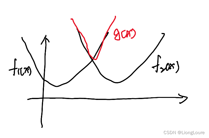
e.g. : suppose f ( x , θ ) f\left( x,\theta \right) f(x,θ) is convex for each θ ∈ [ 1 , 2 ] \theta \in \left[ 1,2 \right] θ∈[1,2] , then g ( x ) = max θ ∈ [ 1 , 2 ] { f ( x , θ ) } g\left( x \right) =\underset{\theta \in \left[ 1,2 \right]}{\max}\left\{ f\left( x,\theta \right) \right\} g(x)=θ∈[1,2]max{f(x,θ)} convex —— f ( x , θ ) = θ x + b f\left( x,\theta \right) =\theta x+b f(x,θ)=θx+b ⇒ \Rightarrow ⇒ g ( x ) = max θ ∈ [ 1 , 2 ] { θ x + b } g\left( x \right) =\underset{\theta \in \left[ 1,2 \right]}{\max}\left\{ \theta x+b \right\} g(x)=θ∈[1,2]max{θx+b}
Pointwise minimum of concave func is concave —— S ( x ) = min θ ∈ [ 1 , 2 ] { θ x + b } S\left( x \right) =\underset{\theta \in \left[ 1,2 \right]}{\min}\left\{ \theta x+b \right\} S(x)=θ∈[1,2]min{θx+b} is concave
4. Short Introduction to Optimization
4.1 Nonlinear Optimiazation Problems
Nonlinear Optimiazation: Primal problem
minimize : f 0 ( x ) f_0\left( x \right) f0(x) —— cost func f : R n → R f:\mathbb{R} ^n\rightarrow \mathbb{R} f:Rn→R , x = [ x 1 ⋮ x n ] ∈ R n x=\left[ \begin{array}{c} x_1\\ \vdots\\ x_{\mathrm{n}}\\ \end{array} \right] \in \mathbb{R} ^n x= x1⋮xn ∈Rn
subject to : f i ( x ) ⩽ 0 , i = 1 , ⋯ , m , h j ( x ) = 0 , j = 1 , ⋯ , q f_{\mathrm{i}}\left( x \right) \leqslant 0,i=1,\cdots ,m , h_{\mathrm{j}}\left( x \right) =0,j=1,\cdots ,q fi(x)⩽0,i=1,⋯,m,hj(x)=0,j=1,⋯,q —— constrain set C = { x ∈ R n : f i ( x ) ⩽ 0 , h j ( x ) = 0 } C=\left\{ x\in \mathbb{R} ^n:f_{\mathrm{i}}\left( x \right) \leqslant 0,h_{\mathrm{j}}\left( x \right) =0 \right\} C={x∈Rn:fi(x)⩽0,hj(x)=0} , if x ∈ C x\in C x∈C , then x x x is called feasible
decison variable x ∈ R n x\in \mathbb{R} ^n x∈Rn , domain D \mathcal{D} D, referred to as primal problem
optimal value p ∗ p^* p∗
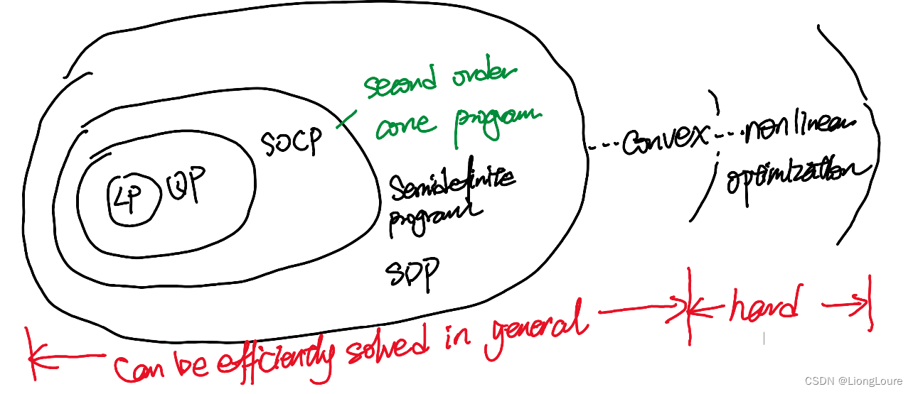
is called a convex optimization problem if f 0 , . . . , f m f_0,...,f_{\mathrm{m}} f0,...,fm are convex and h 1 , . . . , h q h_1,...,h_{\mathrm{q}} h1,...,hq are affine —— means objective function f 0 f_0 f0 is convex and constrain set is convex
typically convex optimization can be solved efficiently
- Categories :
objective func (Linear/affine) + constrain set/func(Linear/affine) —— Linear ProgramLP
objective func (Quardratic - convex) + constrain set/func(Linear/affine) —— Quardratic ProgramQP
objective func (Quardratic - convex) + constrain set/func(uardratic) —— Quardratic Constrained Quardratic ProgramQCQP- Hard to solve
- How to find optimal solutions?
optimality condition: for unconstrained problems : 1st-order optimality condition x ∗ x^* x∗ is local minimizer then ∇ f ( x ∗ ) = 0 \nabla f\left( x^* \right) =0 ∇f(x∗)=0 (Taylor expension)
For convex problem , above condition guarantees x ∗ x^* x∗ is global minimizer
Question : what about constrained optimization?
4.2 Lagrangian
Associated Lagrangian : L : D × R m × R q → R L:\mathcal{D} \times \mathbb{R} ^m\times \mathbb{R} ^q\rightarrow \mathbb{R} L:D×Rm×Rq→R
L ( x , λ , ν ) = f 0 ( x ) + ∑ i = 1 m λ i f i ( x ) + ∑ j = 1 q ν j h j ( x ) , λ i ⩾ 0 , ν j ⩾ 0 L\left( x,\lambda ,\nu \right) =f_0\left( x \right) +\sum_{i=1}^m{\lambda _{\mathrm{i}}f_{\mathrm{i}}\left( x \right)}+\sum_{j=1}^q{\nu _{\mathrm{j}}h_{\mathrm{j}}\left( x \right)},\lambda _{\mathrm{i}}\geqslant 0,\nu _{\mathrm{j}}\geqslant 0 L(x,λ,ν)=f0(x)+i=1∑mλifi(x)+j=1∑qνjhj(x),λi⩾0,νj⩾0
weighted sum of objective and constraints functions
λ i \lambda _{\mathrm{i}} λi : Lagrangian multiplier associated with f i ( x ) ⩽ 0 f_{\mathrm{i}}\left( x \right) \leqslant 0 fi(x)⩽0
ν j \nu _{\mathrm{j}} νj : Lagrangian multiplier associated with h j ( x ) = 0 h_{\mathrm{j}}\left( x \right) =0 hj(x)=0
4.2.1 Lagrangian Dual Problems
Lagrangian Dual Problems : g : R m × R q → R g:\mathbb{R} ^m\times \mathbb{R} ^q\rightarrow \mathbb{R} g:Rm×Rq→R
g ( λ , ν ) = i n f x ∈ D L ( x , λ , ν ) = i n f x ∈ D { f 0 ( x ) + ∑ i = 1 m λ i f i ( x ) + ∑ j = 1 q ν j h j ( x ) } g\left( \lambda ,\nu \right) =\underset{x\in \mathcal{D}}{\mathrm{inf}}L\left( x,\lambda ,\nu \right) =\underset{x\in \mathcal{D}}{\mathrm{inf}}\left\{ f_0\left( x \right) +\sum_{i=1}^m{\lambda _{\mathrm{i}}f_{\mathrm{i}}\left( x \right)}+\sum_{j=1}^q{\nu _{\mathrm{j}}h_{\mathrm{j}}\left( x \right)} \right\} g(λ,ν)=x∈DinfL(x,λ,ν)=x∈Dinf{f0(x)+i=1∑mλifi(x)+j=1∑qνjhj(x)}
- g g g is convex(always true - regardless fo whether the primal peoblem is convex or not) , can be − ∞ -\infty −∞ for some λ , ν \lambda ,\nu λ,ν
- Lower bound property : If λ ⪰ 0 \lambda \succeq 0 λ⪰0 (elementwise) , then g ( λ , ν ) ⩽ p ∗ g\left( \lambda ,\nu \right) \leqslant p^* g(λ,ν)⩽p∗
Let x ~ \tilde{x} x~ be arbitrary feasible primal variable and λ ⩾ 0 \lambda \geqslant 0 λ⩾0 , f 0 ( x ~ ) ⩾ L ( x ~ , λ , ν ) ⩾ i n f x ∈ D L ( x , λ , ν ) = g ( λ , ν ) ⇒ min x ~ f e a s i b l e f 0 ( x ~ ) ⩾ g ( λ , ν ) f_0\left( \tilde{x} \right) \geqslant L\left( \tilde{x},\lambda ,\nu \right) \geqslant \underset{x\in \mathcal{D}}{\mathrm{inf}}L\left( x,\lambda ,\nu \right) =g\left( \lambda ,\nu \right) \Rightarrow \underset{\tilde{x}\,\,feasible}{\min}f_0\left( \tilde{x} \right) \geqslant g\left( \lambda ,\nu \right) f0(x~)⩾L(x~,λ,ν)⩾x∈DinfL(x,λ,ν)=g(λ,ν)⇒x~feasibleminf0(x~)⩾g(λ,ν)
Lagrangian Dual Problems :
maximize : g ( λ , ν ) g\left( \lambda ,\nu \right) g(λ,ν)
subject to : λ ⪰ 0 \lambda \succeq 0 λ⪰0
⇔ \Leftrightarrow ⇔ change convex optimization problem
min : − g ( λ , ν ) -g\left( \lambda ,\nu \right) −g(λ,ν)
subject to : − λ ⪯ 0 -\lambda \preceq 0 −λ⪯0
Fined the best lower bound on p ∗ p^* p∗ using the Lagrange dual function
Dual problem is a convex optimization problem even when the primal is nonconvex
optimal value denoted d ∗ d^* d∗
( λ , ν ) \left( \lambda ,\nu \right) (λ,ν) is called dual feasible if λ ⪰ 0 \lambda \succeq 0 λ⪰0 and ( λ , ν ) ∈ d o m ( g ) \left( \lambda ,\nu \right) \in dom\left( g \right) (λ,ν)∈dom(g)
Often simplified by making the implicit constraint ( λ , ν ) ∈ d o m ( g ) \left( \lambda ,\nu \right) \in dom\left( g \right) (λ,ν)∈dom(g) explicit
例子-见 5
4.2.2 Duality Theorems
- Weak Duality : d ∗ ⩽ p ∗ d^*\leqslant p^* d∗⩽p∗
always hold (for convex and nonconvex problems)
can be used to find nontrivial lower bounds for difficult problems - Strong Duality : d ∗ = p ∗ d^*= p^* d∗=p∗
not true in general, but typically holds for convex problems
conditions that guarantee strong duality in convex problems are called constriant qualifications
Slater’s constraint qualification : Primal is strictly feasible
4.3 General Optimality Conditions
For general optimization problem:
minimize : f 0 ( x ) f_0\left( x \right) f0(x)
subject to : f i ( x ) ⩽ 0 , i = 1 , ⋯ , m , h j ( x ) = 0 , j = 1 , ⋯ , q f_{\mathrm{i}}\left( x \right) \leqslant 0,i=1,\cdots ,m,h_{\mathrm{j}}\left( x \right) =0,j=1,\cdots ,q fi(x)⩽0,i=1,⋯,m,hj(x)=0,j=1,⋯,q
General Optimality Conditions : strong duality and ( x ∗ , λ ∗ , ν ∗ ) \left( x^*,\lambda ^*,\nu ^* \right) (x∗,λ∗,ν∗) is primal-dual optimal ⇔ \Leftrightarrow ⇔
- x ∗ = a r g min x L ( x , λ ∗ , ν ∗ ) x^*=arg\min _{\mathrm{x}}L\left( x,\lambda ^*,\nu ^* \right) x∗=argminxL(x,λ∗,ν∗) —— Lagrange optimality
- λ i ∗ f i ( x ) = 0 , ∀ i \lambda _{\mathrm{i}}^{*}f_{\mathrm{i}}\left( x \right) =0,\forall i λi∗fi(x)=0,∀i —— Complementarity
- f i ( x ∗ ) ⩽ 0 , h j ( x ∗ ) = 0 , ∀ i , j f_{\mathrm{i}}\left( x^* \right) \leqslant 0,h_{\mathrm{j}}\left( x^* \right) =0,\forall i,j fi(x∗)⩽0,hj(x∗)=0,∀i,j —— primal feasibility
- λ i ∗ ⩾ 0 , ∀ i \lambda _{\mathrm{i}}^{*}\geqslant 0,\forall i λi∗⩾0,∀i —— dual feasibility
Proof Necessity
Assume x ∗ x^* x∗ and ( λ ∗ , ν ∗ ) \left( \lambda ^*,\nu ^* \right) (λ∗,ν∗) are primal-dual optimal slns with zero duality gap
f 0 ( x ∗ ) = g ( λ ∗ , ν ∗ ) = min x ∈ D ( f 0 ( x ) + ∑ i = 1 m λ i ∗ f i ( x ) + ∑ j = 1 q ν j ∗ h j ( x ) ) ⩽ f 0 ( x ∗ ) + ∑ i = 1 m λ i ∗ f i ( x ∗ ) + ∑ j = 1 q ν j ∗ h j ( x ∗ ) ⩽ f 0 ( x ∗ ) f_0\left( x^* \right) =g\left( \lambda ^*,\nu ^* \right) =\underset{x\in \mathcal{D}}{\min}\left( f_0\left( x \right) +\sum_{i=1}^m{\lambda _{\mathrm{i}}^{*}f_{\mathrm{i}}\left( x \right)}+\sum_{j=1}^q{\nu _{\mathrm{j}}^{*}h_{\mathrm{j}}\left( x \right)} \right) \leqslant f_0\left( x^* \right) +\sum_{i=1}^m{\lambda _{\mathrm{i}}^{*}f_{\mathrm{i}}\left( x^* \right)}+\sum_{j=1}^q{\nu _{\mathrm{j}}^{*}h_{\mathrm{j}}\left( x^* \right)}\leqslant f_0\left( x^* \right) f0(x∗)=g(λ∗,ν∗)=x∈Dmin(f0(x)+i=1∑mλi∗fi(x)+j=1∑qνj∗hj(x))⩽f0(x∗)+i=1∑mλi∗fi(x∗)+j=1∑qνj∗hj(x∗)⩽f0(x∗)
Therefore, all inequalities are actually equalities
Replacing the first inequality with equality ⇒ x ∗ = a r g min x L ( x , λ ∗ , ν ∗ ) \Rightarrow x^*=arg\min _{\mathrm{x}}L\left( x,\lambda ^*,\nu ^* \right) ⇒x∗=argminxL(x,λ∗,ν∗)
Replacing the second inequality with equality ⇒ \Rightarrow ⇒ complementarity condition
Proof of Sufficiency
Assume ( x ∗ , λ ∗ , ν ∗ ) \left( x^*,\lambda ^*,\nu ^* \right) (x∗,λ∗,ν∗) satisfies the optimality conditions :
g ( λ ∗ , ν ∗ ) = f ( x ∗ ) + ∑ i = 1 m λ i ∗ f i ( x ∗ ) + ∑ j = 1 q ν j ∗ h j ( x ∗ ) = f ( x ∗ ) g\left( \lambda ^*,\nu ^* \right) =f\left( x^* \right) +\sum_{i=1}^m{\lambda _{\mathrm{i}}^{*}f_{\mathrm{i}}\left( x^* \right)}+\sum_{j=1}^q{\nu _{\mathrm{j}}^{*}h_{\mathrm{j}}\left( x^* \right)}=f\left( x^* \right) g(λ∗,ν∗)=f(x∗)+i=1∑mλi∗fi(x∗)+j=1∑qνj∗hj(x∗)=f(x∗)
The first equality is by Lagrange optimality, and the 2nd equality is due to conplementarity
Therefore, the duality gap is zero, and ( x ∗ , λ ∗ , ν ∗ ) \left( x^*,\lambda ^*,\nu ^* \right) (x∗,λ∗,ν∗) is the primal dual optimal solution
4.4 KKT Conditions
For convex optimization problem:
minimize : f 0 ( x ) f_0\left( x \right) f0(x)
subject to : f i ( x ) ⩽ 0 , i = 1 , ⋯ , m , h j ( x ) = 0 , j = 1 , ⋯ , q f_{\mathrm{i}}\left( x \right) \leqslant 0,i=1,\cdots ,m,h_{\mathrm{j}}\left( x \right) =0,j=1,\cdots ,q fi(x)⩽0,i=1,⋯,m,hj(x)=0,j=1,⋯,q
Suppose duality gap is zero , then ( x ∗ , λ ∗ , ν ∗ ) \left( x^*,\lambda ^*,\nu ^* \right) (x∗,λ∗,ν∗) is primal-dual optimal if and only if it satisfies the Karush-Kuhn-Tucker(KKT) conditions
- ∂ L ∂ x ( x , λ ∗ , ν ∗ ) = 0 \frac{\partial L}{\partial x}\left( x,\lambda ^*,\nu ^* \right) =0 ∂x∂L(x,λ∗,ν∗)=0 —— Stationarity
- λ i ∗ f i ( x ∗ ) = 0 , ∀ i \lambda _{\mathrm{i}}^{*}f_{\mathrm{i}}\left( x^* \right) =0,\forall i λi∗fi(x∗)=0,∀i —— Complementarity
- f i ( x ∗ ) ⩽ 0 , h j ( x ∗ ) = 0 , ∀ i , j f_{\mathrm{i}}\left( x^* \right) \leqslant 0,h_{\mathrm{j}}\left( x^* \right) =0,\forall i,j fi(x∗)⩽0,hj(x∗)=0,∀i,j —— primal feasibility
- λ i ∗ ⩾ 0 , ∀ i \lambda _{\mathrm{i}}^{*}\geqslant 0,\forall i λi∗⩾0,∀i —— dual feasibility
5. Linear Program
Primal Formulations
minimize : c T x c^{\mathrm{T}}x cTx
subject to : A x + b , x ⩾ 0 Ax+b,x\geqslant 0 Ax+b,x⩾0
Lagrangian func : L ( x , λ , ν ) = c T x + λ T ( − x ) + ν T ( A x − b ) L\left( x,\lambda ,\nu \right) =c^{\mathrm{T}}x+\lambda ^{\mathrm{T}}\left( -x \right) +\nu ^{\mathrm{T}}\left( Ax-b \right) L(x,λ,ν)=cTx+λT(−x)+νT(Ax−b)
⇒ g ( λ , ν ) = i n f x ∈ R n { ( c T − λ T + ν T A ) x − ν T b } = { − ∞ i f c T − λ T + ν T A ≠ 0 − b T ν i f c T − λ T + ν T A = 0 \Rightarrow g\left( \lambda ,\nu \right) =\underset{x\in \mathbb{R} ^n}{\mathrm{inf}}\left\{ \left( c^{\mathrm{T}}-\lambda ^{\mathrm{T}}+\nu ^{\mathrm{T}}A \right) x-\nu ^{\mathrm{T}}b\,\, \right\} =\begin{cases} -\infty if\,\,c^{\mathrm{T}}-\lambda ^{\mathrm{T}}+\nu ^{\mathrm{T}}A\ne 0\\ -b^{\mathrm{T}}\nu \,\, if\,\,c^{\mathrm{T}}-\lambda ^{\mathrm{T}}+\nu ^{\mathrm{T}}A=0\\ \end{cases} ⇒g(λ,ν)=x∈Rninf{(cT−λT+νTA)x−νTb}={−∞ifcT−λT+νTA=0−bTνifcT−λT+νTA=0
⇒ max λ , ν g ( λ , ν ) \Rightarrow \underset{\lambda ,\nu}{\max}g\left( \lambda ,\nu \right) ⇒λ,νmaxg(λ,ν) , subject to : λ ⩾ 0 , c T − λ T + ν T A = 0 \lambda \geqslant 0,c^{\mathrm{T}}-\lambda ^{\mathrm{T}}+\nu ^{\mathrm{T}}A=0 λ⩾0,cT−λT+νTA=0
Its Dual:
maximize : − b T ν -b^{\mathrm{T}}\nu −bTν
subject to : A T ν + c ⩾ 0 A^{\mathrm{T}}\nu +c\geqslant 0 ATν+c⩾0
- n n n variables q q q equality constraint n n n inequalities ⇒ \Rightarrow ⇒ q q q variables n n n inequalities constraint
6. Quadratic Program
Unconstrained Quadratic Program : Least Squares
minimize : J ( x ) = 1 2 x T Q x + q T x + q 0 J\left( x \right) =\frac{1}{2}x^{\mathrm{T}}Qx+q^{\mathrm{T}}x+q_0 J(x)=21xTQx+qTx+q0
Problem is convex iff Q ⪰ 0 Q\succeq 0 Q⪰0
When J J J is convex , it can be wrtitten as : J ( x ) = ∥ Q 1 2 x − y ∥ 2 + c J\left( x \right) =\left\| Q^{\frac{1}{2}}x-y \right\| ^2+c J(x)= Q21x−y 2+c
KKT condition
Optimal solution


